Simple tone pips

Demonstration of how to generate a simple tone pip.

import matplotlib.pyplot as plt
import numpy as np

from psiaudio import calibration, stim, util

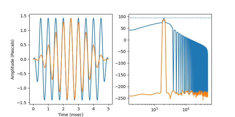
Since 1 Pascal is 94 dB SPL, this calibration results in the stimulus waveform being scaled such that 1 Vrms = 1 Pascal.

cal = calibration.FlatCalibration.from_spl(94)
fs = 100e3

Stimulus levels are always specified in RMS power, not peak-equivalent power. This means that you will see the peak-to-peak tone amplitude run from -1.4 to 1.4 (resulting in a RMS value of 1).

tone1 = stim.ramped_tone(
    fs=fs,
    duration=5e-3,
    rise_time=0.5e-3,
    frequency=2e3,
    level=94,
    calibration=cal,
)

The default value for rise_time is None, which indicates that there’s no plateau (i.e., steady state) period.

tone2 = stim.ramped_tone(
    fs=fs,
    duration=5e-3,
    frequency=2e3,
    level=94,
    calibration=cal,
)


t = np.arange(len(tone1)) / fs * 1e3
psd1 = util.patodb(util.psd_df(tone1, fs))
psd2 = util.patodb(util.psd_df(tone2, fs))

figure, axes = plt.subplots(1, 2, figsize=(8, 4))
axes[0].plot(t, tone1, label='0.5 msec rise/fall')
axes[0].plot(t, tone2, label='2.5 msec rise/fall')

axes[0].set_xlabel('Time (msec)')
axes[0].set_ylabel('Amplitude (Pascals)')

axes[1].semilogx(psd1, label='0.5 msec rise/fall')
axes[1].semilogx(psd2, label='2.5 msec rise/fall')
axes[1].axhline(94, ls=':')

<matplotlib.lines.Line2D object at 0x7fe0921a4a50>

Format the axes. Note the use of psiaudio’s custom scale to show ticks on an octave scale.

axes[1].set_xscale('octave')
axes[1].axis(xmin=250, xmax=16e3, ymin=0, ymax=100)
axes[1].set_xlabel('Frequency (kHz)')
axes[1].set_ylabel('Amplitude (dB SPL)')
axes[1].legend()

figure.tight_layout()

plt.show()