Generate FM, AM and SFM stimuli

This demonstrates how to generate amplitude, frequency, and spectrotemporal modulated stimuli.

import matplotlib.pyplot as plt
import numpy as np

from psiaudio import stim
from psiaudio import util
from psiaudio.calibration import FlatCalibration


def plot_waveform(w, fs):
    figure, axes = plt.subplots(1, 3, figsize=(8, 8/3), constrained_layout=True)
    t = np.arange(len(w)) / fs
    axes[0].plot(t, w)
    axes[0].set_xlabel('Time (sec)')
    axes[0].set_ylabel(f'Amplitude (Pa)')
    axes[1].set_xlabel('Time (sec)')
    axes[1].set_ylabel('Frequency (kHz)')
    axes[1].specgram(w, Fs=fs);
    axes[1].set_yscale('octave', octaves=0.5)
    axes[1].axis(ymin=2e3, ymax=8e3, xmin=0, xmax=1)
    axes[2].plot(util.patodb((util.psd_df(w, fs=fs)).iloc[1:]))
    axes[2].set_xlabel('Frequency (kHz)')
    axes[2].set_ylabel('Amplitude (dB SPL)')
    axes[2].set_xscale('octave', octaves=0.5)
    axes[2].axis(ymin=0, xmin=2e3, xmax=8e3)
    return figure, axes

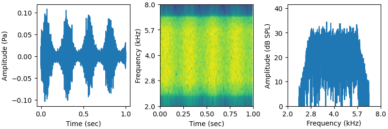
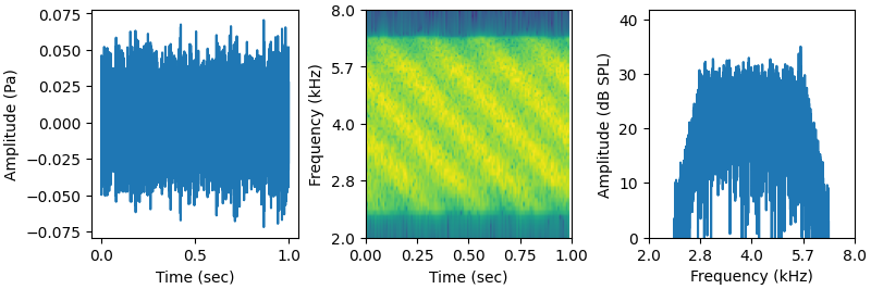
The AM and STM noise can both be generated using the stm function. The difference is in the cpo (cycles per octave) being set to 0 for modulations only in the time domain.

fs = 16000

Add a taper to the rolloff.

frequency = {
    'fc': 4e3,
    'octaves': 1,
    'rolloff_octaves': 0.25,
    'rolloff': 16,
}

w_stm = stim.stm(
    fs=fs,
    frequency=frequency,
    depth=9,
    duration=1,
    cpo=2,
    cps=4,
    mod_type='exp',
    calibration=FlatCalibration.from_spl(94),
    level=60,
)

w_am = stim.stm(
    fs=fs,
    frequency=frequency,
    depth=9,
    duration=1,
    cpo=0,
    cps=4,
    mod_type='exp',
    calibration=FlatCalibration.from_spl(94),
    level=60,
)

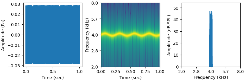
w_fm = stim.sfm(fs, 4e3, 4, 100, 1, 60, FlatCalibration.from_spl(94))

plot_waveform(w_fm, fs)
plot_waveform(w_am, fs)
plot_waveform(w_stm, fs)
plt.show()

• 
• 
•