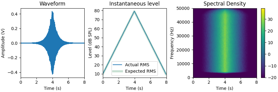
Generate noise linearly ramped in dB

This demonstrates how to generate a bandlimited noise that is ramped linearly at a fixed rate in dB per second.

from matplotlib import pyplot as plt
import numpy as np
from numpy.lib.stride_tricks import sliding_window_view

from scipy.signal import stft

from psiaudio.calibration import FlatCalibration
from psiaudio.stim import EnvelopeFactory, BandlimitedFIRNoiseFactory

from psiaudio import util

Define some basic parameters. The noise will be ramped from 0 dB SPL to max_level at the given ramp_rate. Sweep duration is defined by the max noise level and ramp rate.

The calibration is set such that 1 Vrms = 1 Pa.

fs = 100e3
calibration = FlatCalibration.from_spl(94)

min_level = 10
max_level = 80   # max level for testing
ramp_rate = 17.5 # dB/s

sweep_duration = (max_level - min_level) / ramp_rate * 2

Assemble the factories that will generate the noise. The bartlett envelope is a triangular envelope. Since the envelope operates on the waveform, which is in units of Vrms, we need to apply an exponential transform to achieve the equivalent scaling for the dB domain.

noise = BandlimitedFIRNoiseFactory(
    fs=fs,
    fl=4e3,
    fh=45.2e3,
    level=max_level,
    calibration=calibration,
)


stim = EnvelopeFactory(
    envelope='bartlett',
    fs=fs,
    duration=sweep_duration,
    rise_time=None,
    transform=lambda x: util.dbi((max_level-min_level) * (x - 1)),
    input_factory=noise,
)


figure, axes = plt.subplots(1, 3, figsize=(9, 3), constrained_layout=True,
                            sharex=True)

s = stim.get_samples_remaining()
t = np.arange(len(s)) / fs
axes[0].plot(t, s)
axes[0].set_xlabel('Time (s)')
axes[0].set_ylabel('Amplitude (V)')

window_size = int(0.05 * fs)
window_step = window_size // 10
sv = sliding_window_view(s, window_size)
s_rms = util.rms(sv[::window_step])
s_spl = util.patodb(s_rms)
t_window = np.arange(len(s_spl)) * window_step / fs
axes[1].plot(t_window, s_spl, label='Actual RMS')

i = np.argmax(s_spl)
peak_time = t_window[i]
peak = s_spl[i]
expected = np.abs(t_window - peak_time) * -ramp_rate + peak
axes[1].plot(t_window, expected, color='seagreen', ls='-', lw=5, alpha=0.25, label='Expected RMS')
axes[1].set_xlabel('Time (s)')
axes[1].set_ylabel('Level (dB SPL)')
axes[1].legend()

f, t, Zxx = stft(s, fs, scaling='psd')
spectrum = util.patodb(np.abs(Zxx))
extent = (t.min(), t.max(), f.min(), f.max())
im = axes[2].imshow(spectrum, aspect='auto', extent=extent, origin='lower', vmin=-20)
figure.colorbar(im, ax=axes[2])
axes[2].set_xlabel('Time (s)')
axes[2].set_ylabel('Frequency (Hz)')

axes[0].set_title('Waveform')
axes[1].set_title('Instantaneous level')
axes[2].set_title('Spectral Density')

plt.show()