Queue ordering options

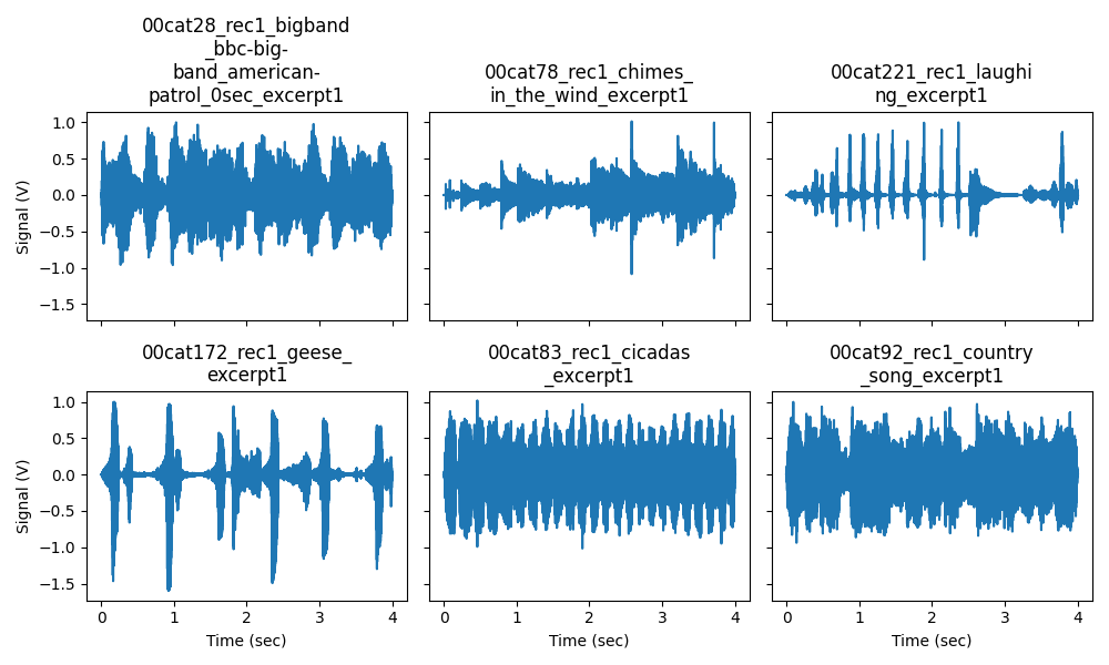
Using a sequence of wav files, we can demonstrate the various ordering options. For all demonstrates, we assume that three trials each of six stimuli (A, B, C, D, E, and F) have been queued.

import textwrap

import matplotlib.pyplot as plt
import numpy as np
from scipy import signal

from psiaudio.stim import wavs_from_path
from psiaudio.queue import (BlockedRandomSignalQueue, BlockedFIFOSignalQueue,
                            GroupedFIFOSignalQueue, FIFOSignalQueue)

First, let’s load the wav files. A utility function is provided that scans a particular folder for all wav files and returns a list of WavFile instances (i.e., a subclass of Waveform). Queues require all stimuli to be a subclass of Waveform).

fs = 100e3
base_path = '../wav-files'
wavfiles = wavs_from_path(fs, base_path)

# Plot each waveform to illustrate what the individual stimuli look like.
figure, axes = plt.subplots(2, 3, figsize=(10, 6), sharex=True, sharey=True)
for ax, w in zip(axes.flat, wavfiles):
    w.reset()
    waveform = w.get_samples_remaining()
    t = np.arange(waveform.shape[-1]) / w.fs
    ax.plot(t, waveform)
    title = textwrap.fill(w.filename.stem, 20)
    ax.set_title(title)

for ax in axes[:, 0]:
    ax.set_ylabel('Signal (V)')
for ax in axes[-1]:
    ax.set_xlabel('Time (sec)')

figure.tight_layout()

Now, calculate how many samples we want to pull out of the queue on each call to AbstractSignalQueue.pop_buffer.

n_samples = sum(w.n_samples() for w in wavfiles)

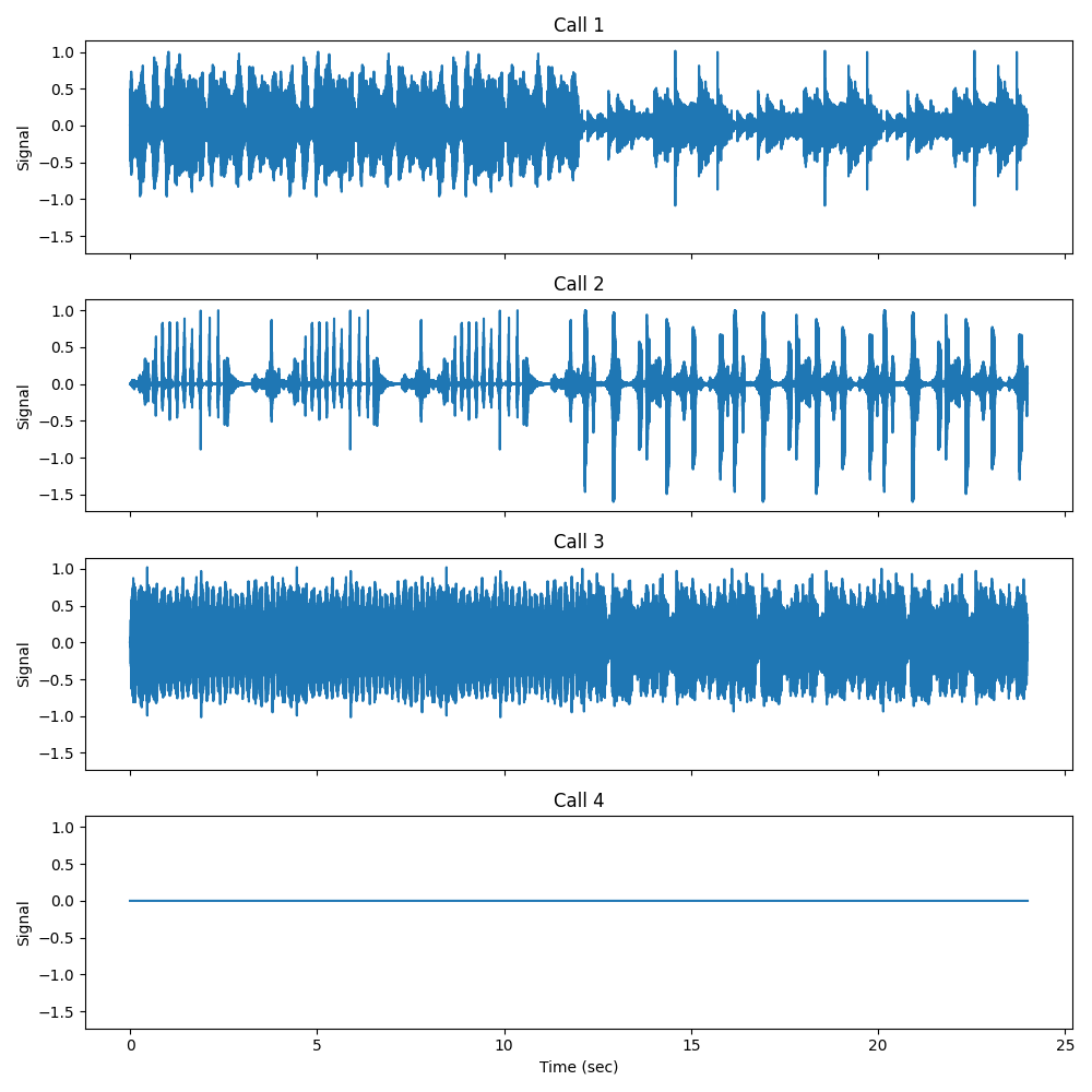
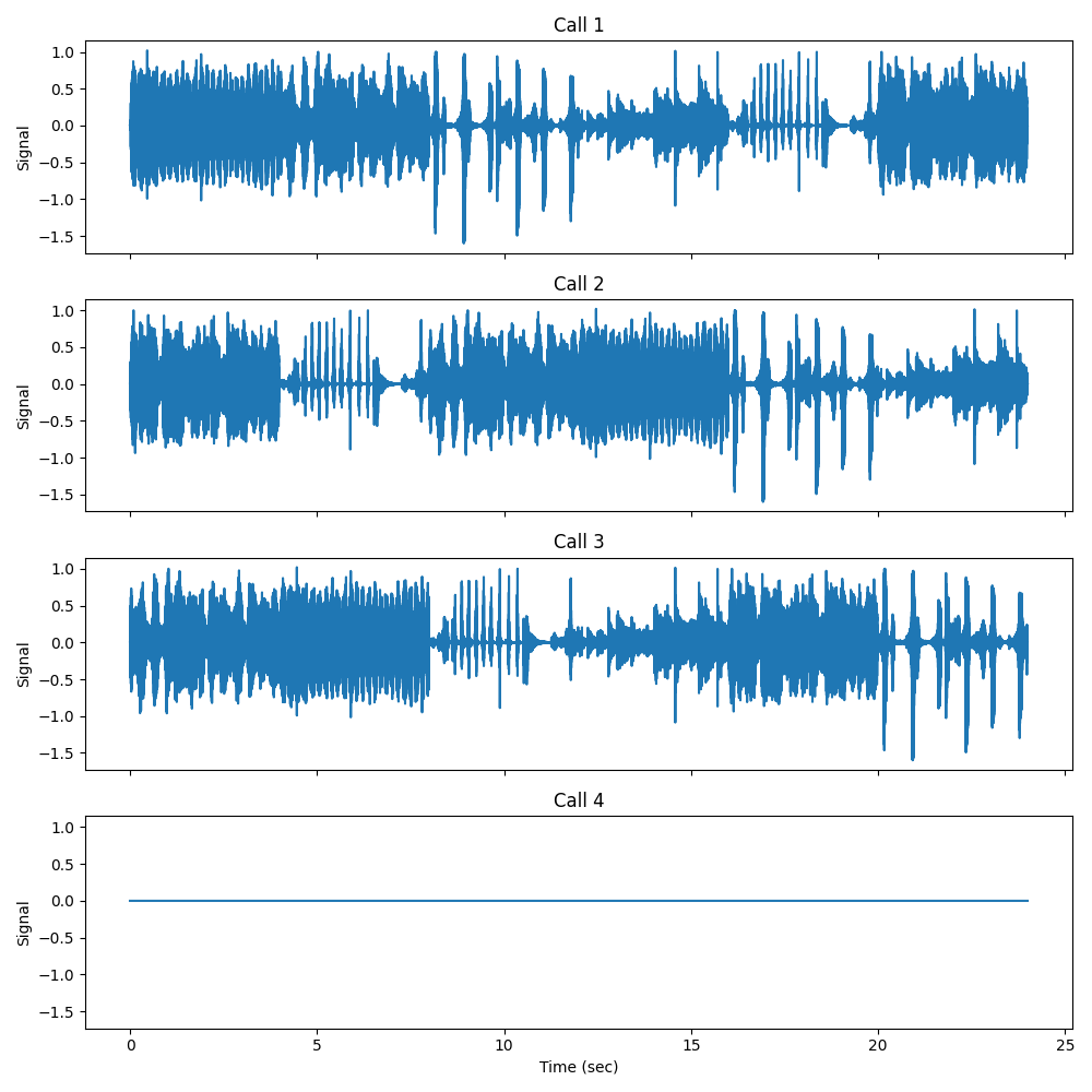
We also create a utility function to plot the queue contents. This function calls queue.pop_buffer six times and plots the result. These samples can be used, for example, to “feed” the portaudio output buffer which has a callback that requests a fresh number of samples at a fixed interval. Note that the final call returns a sequence of zeros since we have presented the requested number of trials for each stimuli.

def plot_queue(queue, n_samples):
    t = np.arange(n_samples) / queue.fs
    figure, axes = plt.subplots(4, 1, figsize=(10, 10), sharex=True,
                                sharey=True)
    for i, ax in enumerate(axes.flat):
        waveform = queue.pop_buffer(n_samples)
        ax.plot(t, waveform)
        ax.set_title(f'Call {i+1}')
        ax.set_ylabel('Signal')
    axes[-1].set_xlabel('Time (sec)')
    figure.tight_layout()

The most basic queue is FIFOSignalQueue. The first stimulus is presented for the specified number of trials before advancing to the next stimuli. The ordering of the stimuli will be:

A A A B B B C C C D D D E E E F F F

queue = FIFOSignalQueue(fs=fs)
queue.extend(wavfiles, trials=3)
plot_queue(queue, n_samples)

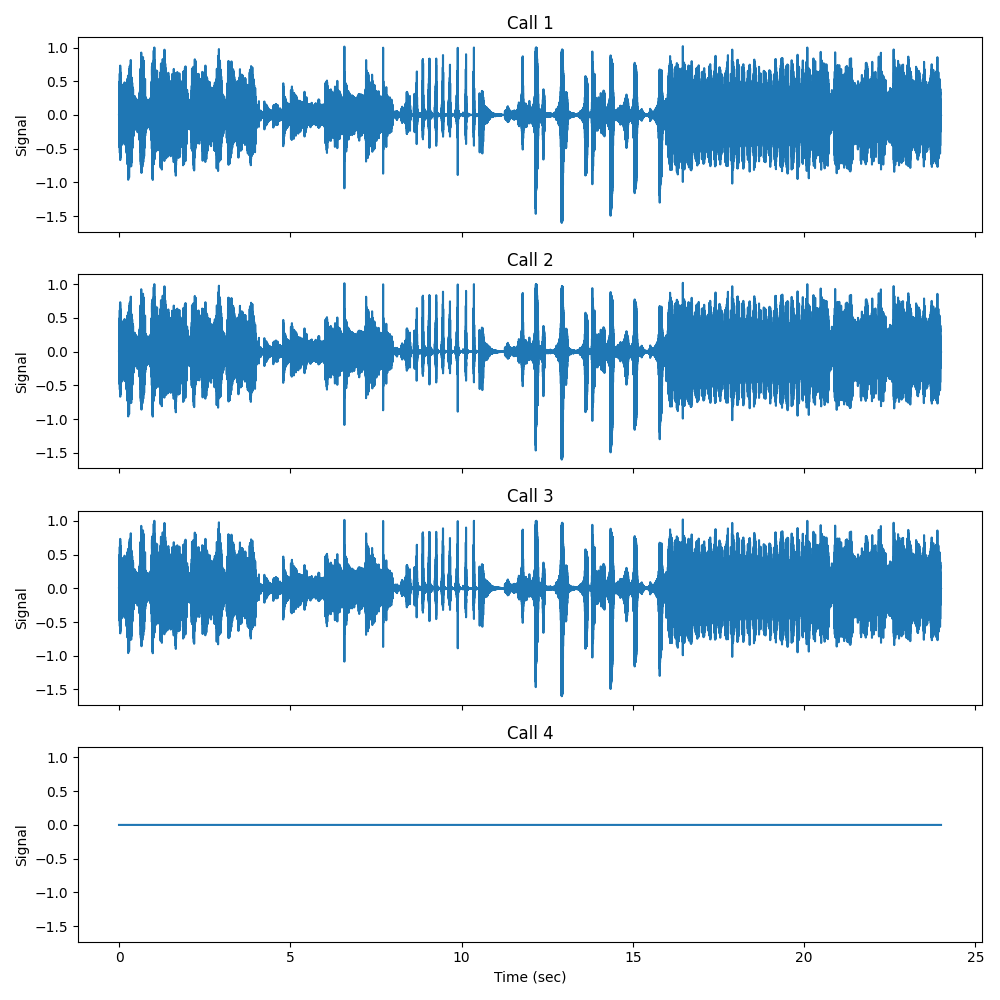
The next type of queue is BlockedFIFOSignalQueue. The stimuli are interleaved (in the order they were queued). All stimuli are presented before advancing to the next trial.

A B C D E F A B C D E F A B C D E F

queue = BlockedFIFOSignalQueue(fs=fs)
queue.extend(wavfiles, 3)
plot_queue(queue, n_samples)

To modify the block size, use GroupedFIFOSignalQueue. Like BlockedFIFO stimuli will be presented in groups, but you can manually set the group size to create sub-blocks that are presented before advancing to the next sublock. In the following example, the group size is 3, creating two sub-blocks:

A B C A B C A B C D E F D E F D E F

queue = GroupedFIFOSignalQueue(group_size=3, fs=fs)
queue.extend(wavfiles, 3)
plot_queue(queue, n_samples)

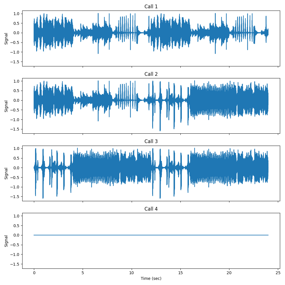
We can also randomize stimuli within each block using BlockedRandomSignalQueue.

queue = BlockedRandomSignalQueue(fs=fs)
queue.extend(wavfiles, 3)
plot_queue(queue, n_samples)

plt.show()