Note
Go to the end to download the full example code.
Generate stimuli with gaps
This demonstrates how to generate various stimuli with gaps (e.g., for measuring temporal processing).
import matplotlib.pyplot as plt
import numpy as np

from psiaudio import calibration
from psiaudio import stim
from psiaudio import util


# Creating calibration
# --------------------
# This ensures that the resulting waveform is in units of Pascals.
flat_cal = calibration.FlatCalibration.from_spl(94)
fs = 100e3
Narrowband noise with gap
Gap embedded in narrowband noise.
waveform = stim.gap(
    fs=fs,
    fc=1e3,
    octaves=1/8,
    filter_rolloff=1/4,
    gap=8e-3,
    durations=[32e-3, 32e-3],
    rise_time=2e-3,
    level=80,
    calibration=flat_cal,
    use_sos=True,
)

t = np.arange(len(waveform)) / fs
figure, axes = plt.subplots(1, 3, figsize=(9, 3), constrained_layout=True)
axes[0].plot(t, waveform)
axes[0].set_xlabel('Time (s)')
axes[1].set_xlabel('Amplitude (Pa)')
axes[1].specgram(waveform, Fs=fs);
axes[1].axis(ymin=200, ymax=64e3)
axes[1].set_yscale('octave', octaves=2)
axes[0].set_xlabel('Time (s)')
axes[1].set_xlabel('Frequency (kHz)')
spl = util.patodb(util.psd_df(waveform, fs=fs))
axes[2].plot(spl.iloc[1:])
axes[2].set_xscale('octave', octaves=2)
axes[2].set_xlabel('Frequency (kHz)')
axes[2].set_ylabel('Level (dB SPL)')
axes[2].axis(ymin=0, ymax=80, xmin=200, xmax=64e3)
axes[2].axhline(80)

plt.show()
/opt/hostedtoolcache/Python/3.13.13/x64/lib/python3.13/site-packages/matplotlib/axes/_axes.py:8283: RuntimeWarning: divide by zero encountered in log10
  Z = 10. * np.log10(spec)
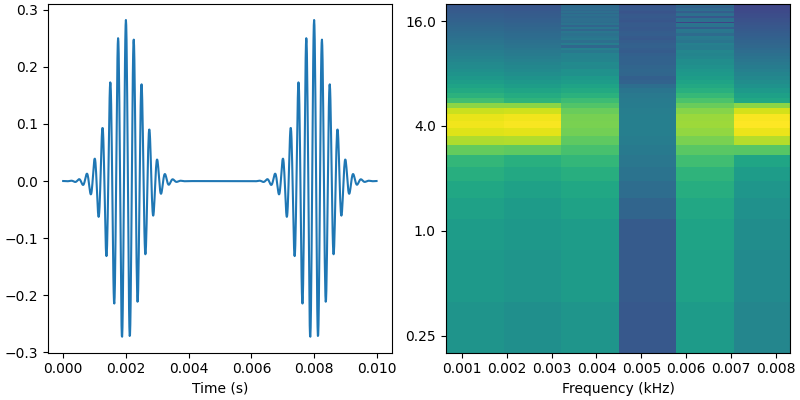
Gap detection based on tone pips
Commonly used in human studies.
waveform = stim.gap(
    fs=fs,
    fc=4e3,
    octaves=0,
    gap=2e-3,
    durations=[4e-3, 4e-3],
    rise_time=2e-3,
    level=80,
    calibration=flat_cal,
)

t = np.arange(len(waveform)) / fs
figure, axes = plt.subplots(1, 2, figsize=(8, 4), constrained_layout=True)
axes[0].plot(t, waveform)
axes[0].set_xlabel('Time (s)')
axes[1].set_xlabel('Amplitude (Pa)')
axes[1].specgram(waveform, Fs=fs);
axes[1].axis(ymin=200, ymax=20e3)
axes[1].set_yscale('octave', octaves=2)
axes[0].set_xlabel('Time (s)')
axes[1].set_xlabel('Frequency (kHz)')
plt.show()
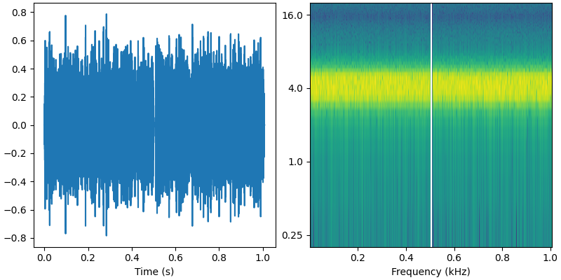
Gap detection based on bandlimited noise
Commonly used in animal studies.
waveform = stim.gap(
    fs=fs,
    fc=4e3,
    octaves=0.5,
    gap=8e-3,
    durations=[500e-3, 500e-3],
    rise_time=2e-3,
    level=80,
    calibration=flat_cal,
)

t = np.arange(len(waveform)) / fs
figure, axes = plt.subplots(1, 2, figsize=(8, 4), constrained_layout=True)
axes[0].plot(t, waveform)
axes[0].set_xlabel('Time (s)')
axes[1].set_xlabel('Amplitude (Pa)')
axes[1].specgram(waveform, Fs=fs);
axes[1].axis(ymin=200, ymax=20e3)
axes[1].set_yscale('octave', octaves=2)
axes[0].set_xlabel('Time (s)')
axes[1].set_xlabel('Frequency (kHz)')
plt.show()
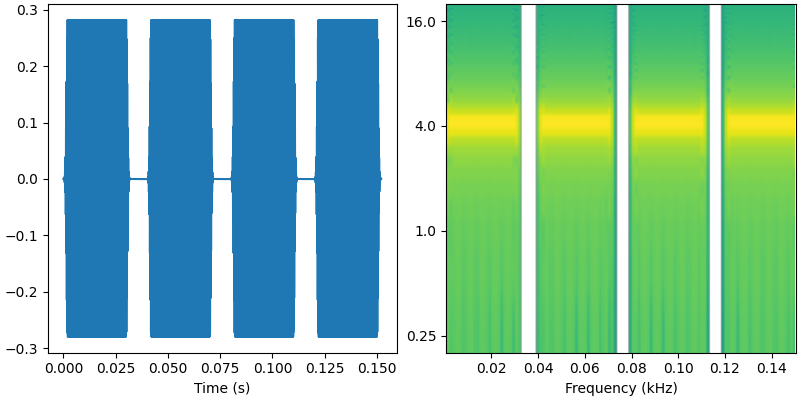
Multiple gaps based on tone pips
Commonly used in animal studies to help train the animal before switching to a single gap. This embeds three gaps in the stimulus.
waveform = stim.gap(
    fs=fs,
    fc=4e3,
    octaves=0,
    gap=8e-3,
    durations=[32e-3, 32e-3, 32e-3, 32e-3],
    rise_time=2e-3,
    level=80,
    calibration=flat_cal,
)

t = np.arange(len(waveform)) / fs
figure, axes = plt.subplots(1, 2, figsize=(8, 4), constrained_layout=True)
axes[0].plot(t, waveform)
axes[0].set_xlabel('Time (s)')
axes[1].set_xlabel('Amplitude (Pa)')
axes[1].specgram(waveform, Fs=fs);
axes[1].axis(ymin=200, ymax=20e3)
axes[1].set_yscale('octave', octaves=2)
axes[0].set_xlabel('Time (s)')
axes[1].set_xlabel('Frequency (kHz)')
plt.show()

Total running time of the script: (0 minutes 0.921 seconds)