Calibration basics

This demonstrates how the calibration classes work.

from matplotlib import pylab as plt
import numpy as np
from scipy import signal

from psiaudio.calibration import FlatCalibration, InterpCalibration
from psiaudio import stim

The core of each calibration class is a sensitivity attribute that represents the output (or input) of the device in dB(Vrms/Pa).

Let’s assume that a 1 Vrms tone generates 1 Pascal (i.e., 94 dB SPL). The sensitivity is then $20 cdot log_{10} (frac{1 V_{RMS}}{20 mu Pa})$.

calibration = FlatCalibration(sensitivity=20*np.log10(1/20e-6))

The calibration instance has many methods that can be used to get relevant numbers. For example, Calibration.get_sf(frequency, level) returns the amplitude (in Vrms) required for generating a tone of the given level (sf is short for scale factor).

for level in (74, 94, 114):
    amplitude = calibration.get_sf(1e3, level)
    print(f'{level:>3d} dB SPL tone should be {amplitude:.1f} Vrms')

 74 dB SPL tone should be 0.1 Vrms
 94 dB SPL tone should be 1.0 Vrms
114 dB SPL tone should be 10.0 Vrms

An instance of FlatCalibration assumes that the output (or input) device has a uniform frequency response.

for frequency in (1e3, 2e3, 4e3, 8e3):
    amplitude = calibration.get_sf(frequency, 114)
    print(f'{frequency*1e-3:.0f} kHz tone should be {amplitude:.1f} Vrms')

1 kHz tone should be 10.0 Vrms
2 kHz tone should be 10.0 Vrms
4 kHz tone should be 10.0 Vrms
8 kHz tone should be 10.0 Vrms

There are several helper methods that make it easy to create a calibration. Two are designed to work with units of dB SPL:

• Calibration.from_pascals(magnitude, vrms). Used when you measure the output in Pascals for a stimulus of the specifid Vrms *

• Calibration.from_spl(spl, vrms). Used when you measure the output, in dB SPL, for a stimulus of the specified Vrms.

Let’s assume that you generate a 0.1 Vrms tone and measure the output as 80 dB SPL.

calibration = FlatCalibration.from_spl(spl=80, vrms=0.1)
for level in (60, 80, 100):
    amplitude = calibration.get_sf(1e3, level)
    print(f'{level:>3d} dB SPL tone should be {amplitude:.2f} Vrms')

 60 dB SPL tone should be 0.01 Vrms
 80 dB SPL tone should be 0.10 Vrms
100 dB SPL tone should be 1.00 Vrms

If you have a speaker where the output that varies with frequency, you can use the InterpCalibration class with an array of frequencies and sensitivities. Assume that SPL is measured using a 1 Vrms tone

frequency =    np.array([500, 1000, 2000, 4000, 8000, 16000])
measured_SPL = np.array([ 80,   90,  100,  100,   90,    80])

calibration = InterpCalibration(frequency=frequency, sensitivity=measured_SPL)

Now, get the required tone amplitude (in Vrms) to generate a 90 dB SPL tone for each frequency.

amplitude = calibration.get_sf(frequency, 90)
for f, a in zip(frequency, amplitude):
    print(f'{f*1e-3:>2.0f} kHz tone should be {a:.2f} Vrms')

 0 kHz tone should be 3.16 Vrms
 1 kHz tone should be 1.00 Vrms
 2 kHz tone should be 0.32 Vrms
 4 kHz tone should be 0.32 Vrms
 8 kHz tone should be 1.00 Vrms
16 kHz tone should be 3.16 Vrms

The calibration also works for input devices (i.e., microphones), too! Let’s assume our microphone generates 0.1 Vrms for a 94 dB SPL 1 kHz tone.

calibration = FlatCalibration.from_spl(94, 0.1)
spl = calibration.get_spl(1e3, 0.1)
print(f'An 0.1 Vrms 1 kHz microphone waveform is {spl:.2f} dB SPL')

An 0.1 Vrms 1 kHz microphone waveform is 94.00 dB SPL

The calibration classes make it very easy to get the signal spectrum in dB SPL. Let’s assume that the microphone does not have a flat frequency response. Assume that SPL is measured using a 1 Vrms tone

frequency =     np.array([0,   500, 1000, 2000, 4000, 8000, 16000, 50000])
measured_vrms = np.array([3,   3,   1,    0.3,  0.3,  1,    3,     3])

calibration = InterpCalibration.from_spl(frequency, spl=90, vrms=measured_vrms)

spl = calibration.get_spl(frequency, 1)
for f, s in zip(frequency, spl):
    print(f'1 Vrms {f*1e-3:>2.0f} kHz sine wave is generated by a {s:.2f} dB SPL tone')

1 Vrms  0 kHz sine wave is generated by a 80.46 dB SPL tone
1 Vrms  0 kHz sine wave is generated by a 80.46 dB SPL tone
1 Vrms  1 kHz sine wave is generated by a 90.00 dB SPL tone
1 Vrms  2 kHz sine wave is generated by a 100.46 dB SPL tone
1 Vrms  4 kHz sine wave is generated by a 100.46 dB SPL tone
1 Vrms  8 kHz sine wave is generated by a 90.00 dB SPL tone
1 Vrms 16 kHz sine wave is generated by a 80.46 dB SPL tone
1 Vrms 50 kHz sine wave is generated by a 80.46 dB SPL tone

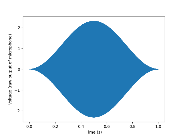
Let’s generate a test signal, a hann-windowed chirp! Let’s assume that chirp is the actual voltage measured by the microphone.

fs = 100e3

chirp = stim.chirp(fs=fs, start_frequency=0.5e3, end_frequency=5e3, duration=1,
                   level=1, window='hann')
t = np.arange(len(chirp)) / fs

plt.plot(t, chirp)
plt.xlabel('Time (s)')
plt.ylabel('Voltage (raw output of microphone)')
plt.show()

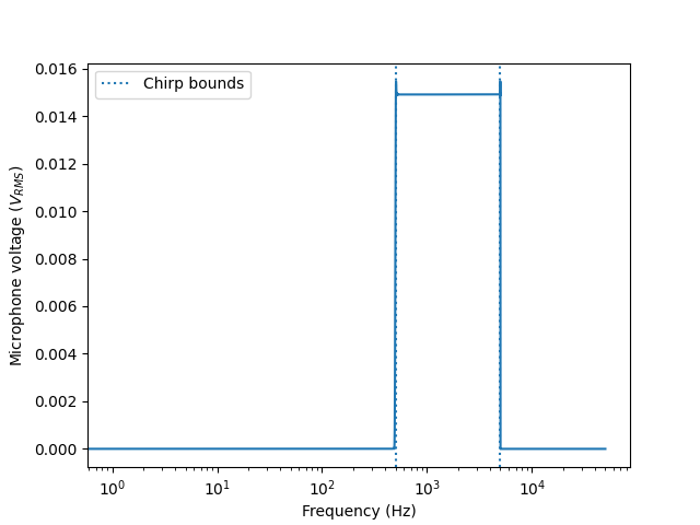
Let’s get the measured Vrms across frequency and plot it.

n = len(chirp)
csd = np.fft.rfft(chirp) / n
psd_vrms = 2 * np.abs(csd) / np.sqrt(2)

freq = np.fft.rfftfreq(n, 1/fs)
plt.semilogx(freq, psd_vrms)
plt.xlabel('Frequency (Hz)')
plt.ylabel('Microphone voltage ($V_{RMS}$)')
plt.axvline(0.5e3, ls=':', label='Chirp bounds')
plt.axvline(5e3, ls=':')
plt.legend()
plt.show()

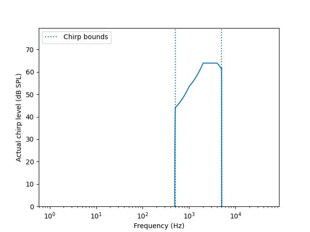
Now that we have our spectrum in Vrms, we can calculate the chirp in dB SPL given the microphone calibration.

spl = calibration.get_spl(freq, psd_vrms)

plt.semilogx(freq, spl)
plt.xlabel('Frequency (Hz)')
plt.ylabel('Actual chirp level (dB SPL)')
plt.axvline(0.5e3, ls=':', label='Chirp bounds')
plt.axvline(5e3, ls=':')
plt.legend()
plt.axis(ymin=0)
plt.show()