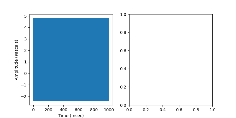
Calibrated multitone complex

This demonstrates how to generate multiple tones of equal SPL when the speaker’s output is not uniform.

import matplotlib.pyplot as plt
import numpy as np

from psiaudio import calibration, stim, util


frequencies = [1e3, 2e3, 4e3, 8e3]
levels =      [ 94,  98,  92, 100]
cal = calibration.InterpCalibration.from_spl(frequencies, levels)

fs = 100e3

We take advantage of Numpy broadcasting to return a 2D array of frequency x time. Each row represents a tone of the desired frequency. By summing across rows, we can get a single stimulus waveform that contains all tone frequencies.

frequencies = np.array(frequencies)[:, np.newaxis]
tone_complex = stim.ramped_tone(
    fs=fs,
    duration=1,
    rise_time=5e-3,
    frequency=frequencies,
    level=94,
    calibration=cal,
)

tone_complex = tone_complex.sum(axis=0)

Calculate an offset such that the tone is centered in the time plot.

t = np.arange(len(tone_complex)) / fs * 1e3

figure, axes = plt.subplots(1, 2, figsize=(8, 4))
axes[0].plot(t, tone_complex)

axes[0].set_xlabel('Time (msec)')
axes[0].set_ylabel('Amplitude (Pascals)')

psd = util.patodb(util.psd_df(tone_complex, fs))

Plot the spectrum. Note the use of psiaudio’s custom scale to show ticks on an octave scale.

axes[1].plot(psd)
axes[1].set_xscale('octave')
axes[1].axis(xmin=250, xmax=16e3, ymin=0, ymax=100)

axes[1].set_xlabel('Frequency (kHz)')
axes[1].set_ylabel('Amplitude (dB SPL)')

figure.tight_layout()

plt.show()