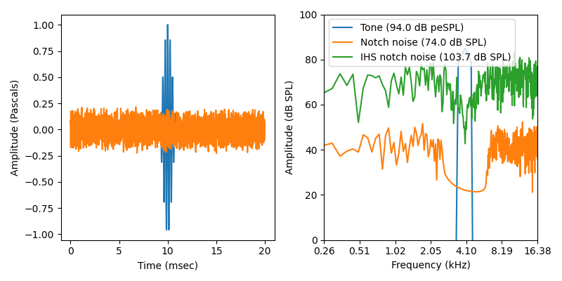
Tones in notch noise

This demonstrates how to generate notch-noise tone pips that can be used for an ABR stimulus.

import matplotlib.pyplot as plt
import numpy as np

from psiaudio import calibration, stim, util


cal = calibration.FlatCalibration.from_spl(94)
fs = 100e3

In human ABRs, duration typically varies with frequency but the number of cycles are fixed.

n_cycles = 8
frequency = 4e3
duration = 8 / 4e3
noise_duration = 20e-3
noise_level = 94-20

Since the calibration scales stimuli to match the requested RMS level, we need to subtract by 3 dB if we want peak-equivalent SPL.

tone = stim.ramped_tone(
    fs=fs,
    duration=duration,
    rise_time=None,
    frequency=frequency,
    level=94 - 3,
    calibration=cal,
)

Notch noise calculations. By dividing or multiplying by the same number, we generate a notch where both sides are equidistant from the target frequency on a log scale.

fl = frequency / 1.5
fh = frequency * 1.5

The gain dictionary must start at 0 Hz and end at Nyquist (i.e., fs/2).

gains = {
    # No attenuation for frequencies below the notch. The transition from no
    # attenuation to full attenuation is specified by fl / 1.1 to fl.
    0: 0,
    fl / 1.1: 0,

    # Attenuate frequencies in the notch by 80 dB.
    fl: -80,
    fh: -80,

    # No attenuation for frequencies above the notch.
    fh * 1.1: 0,
    fs / 2: 0
}


noise = stim.shaped_noise(
    fs=fs,
    gains=gains,
    duration=noise_duration,
    level=noise_level,
    calibration=cal,
)

noise_level = cal.get_spl(None, util.rms(noise))
tone_level = cal.get_spl(frequency, tone.max())

Alternatively, we can use a simple notch like that used by Intelligent Hearing Systems.

# Here, we want to set the noise level such that the spectrum level is 20 dB
# below the peak-equivalent of the tone burst. This is a somewhat complex
# calculation since it requires us to figure out how the noise is divided into
# bins given the noise duration and sampling rate. The number of FFT bins is
# defined as fs / N where N is the number of samples. Since N is equal to
# duration * fs, this simplifies to 1 / duration. Next, we are assuming the
# noise will be fully broadband, so this means the noise will span the full
# range of possible frequencies (0 to Nyquist). By dividing the frequency range
# by the bin width, we get the number of bands the noise is distributed across.
bin_width = 1 / noise_duration
f_max = fs / 2
n_bins = f_max / bin_width
band_level = util.spectrum_to_band_level(94-20, n_bins)

ihs_noise = stim.notch_noise(
    fs=fs,
    notch_frequency=frequency,
    q=1.33,
    level=band_level,
    duration=noise_duration,
    calibration=cal,
)

ihs_noise_level = cal.get_spl(None, util.rms(ihs_noise))

Calculate an offset such that the tone is centeredi n the time plot.

tone_offset = 10e-3 - duration / 2
t_tone = (np.arange(len(tone)) / fs + tone_offset) * 1e3
t_noise = np.arange(len(noise)) / fs * 1e3

psd_tone = util.patodb(util.psd_df(tone, fs))
psd_noise = util.patodb(util.psd_df(noise, fs))
psd_ihs_noise = util.patodb(util.psd_df(ihs_noise, fs))

figure, axes = plt.subplots(1, 2, figsize=(8, 4))
axes[0].plot(t_tone, tone)
axes[0].plot(t_noise, noise)

axes[0].set_xlabel('Time (msec)')
axes[0].set_ylabel('Amplitude (Pascals)')

axes[1].semilogx(psd_tone, label=f'Tone ({tone_level:.1f} dB peSPL)')
axes[1].semilogx(psd_noise, label=f'Notch noise ({noise_level:.1f} dB SPL)')
axes[1].semilogx(psd_ihs_noise, label=f'IHS notch noise ({ihs_noise_level:.1f} dB SPL)')

ticks = util.octave_space(250, 16e3, 1)
axes[1].axis(xmin=ticks[0], xmax=ticks[-1], ymin=0, ymax=100)
axes[1].set_xticks(ticks)
axes[1].set_xticklabels(f'{t*1e-3:.2f}' for t in ticks)
axes[1].set_xticks([], minor=True)
axes[1].set_xlabel('Frequency (kHz)')
axes[1].set_ylabel('Amplitude (dB SPL)')
axes[1].legend()

figure.tight_layout()

plt.show()